Excel has a nifty way to handle situations where you want to add up numbers that don’t match a certain condition. I often find myself reaching for the SUMIF or SUMIFS functions for this. Both are pretty versatile, and they fit different needs depending on what you’re trying to sum. My walk-through is going to cover how to use them, giving you the flexibility to apply these functions effectively.
Thinking back on all the advanced Excel exercises I’ve done, mastering these functions has been a game changer. They can be found in any well-rounded Excel functions file or practice workbook. For those who want to push their Microsoft Excel skills further, getting to know SUMIF and SUMIFS inside out is essential, and I’m excited to share how they’re used in real-world scenarios.
SUMIF Not Equal To
When working with Excel, there are times I need to sum values in a range that don’t meet a specific condition. For such tasks, I use the SUMIF function with the not equal to operator. Here’s how you can use it:
-
Start with the equal sign followed by SUMIF and an open parenthesis:
=SUMIF(. -
Select the criteria_range, which is the range of cells you want to apply the condition to. Say my criteria range is A2.
-
Next, define your condition using the not equal operator (
<>). If I want to exclude the value 2000 from my sum, I enter"<>2000". -
Afterwards, indicate the sum_range. Assuming the cells I want to add up are also in A2, I’d reference the same range again.

-
Simply close the parentheses and press enter to get the sum of cells not equal to 2000.
It’s convenient because if my sum_range is the same as my criteria_range, I can skip it and Excel assumes I’m referring to the criteria_range:
=SUMIF(A2:A14,"<>2000")
This gives me a total of all the values except those equal to 2000. And it looks like my dataset ignores the three times 2000 showed up, as it should.
Bold point: The sum_range is optional; if you don’t specify it, Excel automatically uses the criteria_range for the sum. This keeps my formulas simpler and my worksheets cleaner.
By using SUMIF with the not equal to operator, I effectively exclude specific values and calculate the sum of the remaining numbers swiftly.
SUMIFS Not Equal to Multiple Values (Text)
When I need to sum up quantities in Excel that don’t include specific items—let’s say, products A and C—I use a nifty function called SUMIFS. Here’s how I nail it:
=SUMIFS(B2:B13,A2:A13,"<>A",A2:A13,"<>C")
In my SUMIFS function, B2 is my range with numbers I want to add up, and A2 holds the product names. By setting “< >A” and “< >C” as my criteria1 and criteria2, Excel sums everything except A or C. It’s like telling Excel, “Add these up, but skip A and C, please!”
This method is perfect when I’m juggling multiple values that don’t make my sum cut.
Related Formulas
In my work with Excel, I’ve seen how formulas can be adapted for a wide range of conditions. For instance, using SUMIF accommodates simple requirements like summing values greater than or less than a given number:
- Sum Greater Than:
=SUMIF(range, ">value", sum_range) - Sum Less Than:
=SUMIF(range, "<value", sum_range)
And then, there’s the versatility of SUMIFS for more complex scenarios, which allows for multiple conditions, such as summing values in a date range or based on different criteria using or logic:
- Sum Between Dates:
=SUMIFS(sum_range, date_range, ">=start_date", date_range, "<=end_date") - Using OR logic: Since
SUMIFSis inherently AND logic, for OR logic we need a different approach, possibly summing multipleSUMIFSfor each condition.
Excel doesn’t restrict us to exact matches either. Wildcard characters (*, ?, ~) in SUMIF enable sums based on partial text—super handy for inconsistent datasets:
- Sum with Wildcards:
=SUMIF(range, "text*", sum_range)
While working with numerical datasets, it’s common to handle cells based on their content status:
- Sum Non-Blank:
=SUMIF(range, "<>", sum_range) - Sum Blank:
=SUMIF(range, "=", sum_range)
And if you’re looking to incorporate more than just raw values – perhaps a lookup in your sum formula – combining VLOOKUP with SUMIF comes in as a powerful solution.
Also, I find it particularly flexible to sum values by specific time periods like months or years, which is a breeze using the right functions.
- Sum by Year:
=SUMIF(year_range, year, sum_range) - Sum by Month:
=SUMIF(month_range, month, sum_range)
Remember, when working with text criteria, encapsulate your arguments within double quotes, and for numeric/range criteria, case sensitivity isn’t an issue. As for formulas, understanding the syntax and usage is key to making your dataset yield the answers you need.


