Change Negative Number to Positive: Quick Conversion Tips

In Excel, there’s no shortage of tricks up our sleeves when it comes to managing data. I’ve come across a handy set of methods for an issue that’s quite common for anyone crunching numbers regularly—converting negative numbers to positive ones. Imagine working with financial data, where negative values represent debits or losses. In many cases, you may find yourself needing to flip those figures into positive territory, whether for a high-level presentation or simply to make your datasets more digestible.

Now, not only can these conversion techniques help clean up your spreadsheets, but they also enhance data analysis. By mastering a variety of formulas and understanding the functionality of tools like pivot tables, you’ll be able to transform your data in no time. Just recently, I discovered there are seven different ways to tackle this very issue, each with its own flavor, making use of Excel’s robust feature set—from the generic formula application to the adept use of pivot tables and charts, ensuring that your numbers accurately reflect the values you need to analyze.

1. Multiply with Minus One to Convert a Positive Number

Turning a negative number into a positive is straightforward in Excel. I just multiply it by -1. It’s like giving negativity a high five that flips it into a cheer. For example, if I’ve got -5 in a cell, I punch in:

=my_negative_number*-1

Suddenly, it’s a shiny +5. Here’s a step-by-step run-through:

• Enter -1 in a cell next to the row of negative numbers.
• Use this formula: =negative_value*-1 in the cell adjacent to the first negative number.
• Drag the formula down to convert all cells in the range.

When positive and negative numbers are mixed together, I tweak my approach:

• Input: =IF(A1 < 0, A1*-1, A1) in the cell next to the mixed number.
• Copy and paste this formula for all relevant cells.

Smart use of the IF function keeps the positive numbers unchanged while the negative ones flip to positive. It’s like Excel is a DJ, remixing all the negative hits into positive vibes.

2. Convert to an Absolute Number with ABS Function

In Excel, flipping a negative to a positive is a no-brainer with the ABS function. Think of it as the bouncer that tosses out negative signs, leaving you with just the number’s value—no fuss about whether it’s positive or negative.

Here’s an easy guide:

• Type =ABS(A2) right beside your negative number in cell A2.
• Drag the formula down to convert the whole column.

The formula looks like:

=ABS(number)

If I’ve got a mix of both positive and negative numbers, I don’t sweat it. The ABS function neatly ignores those already positive, focusing only on flipping the negatives.

Now, imagine a column of negative numbers from A2 to A11. I just use =ABS(A2) in B2, copy it down to B11, and like magic, negatives turn positive.

3. Multiple Using Paste Special

Making negative numbers positive in the same Excel column is a breeze with the Paste Special feature. Here’s how I get it done without a sweat:

• I start by typing -1 in any cell and copy it (Ctrl+C).
• Then, I highlight the cells with the negative figures.
• I right-click to bring up the menu and select Paste Special.
• Under the Operations section, “Multiply” is my go-to option.
• Hitting OK, and just like magic, all those pesky negatives flip to positives.

Just note that this isn’t a once-and-done thing; it’s not dynamic. If any new data comes in, I roll up my sleeves and do it all over again. Still, it’s a nifty shortcut that saves me from extra formulae and columns.

4. Remove the Negative Sign with Flash Fill

Flash Fill in Excel is a pretty nifty feature I often use to quickly adjust data. Let’s say I have a bunch of negative numbers that I’d rather see in their positive form. Here’s how I make that happen:

1. I start by typing the positive version of the first negative number into the adjacent cell. For example, if A2 is -100, I’ll type 100 into B2.
2. Next, I move to cell B3 and press Ctrl + E. This triggers Flash Fill to recognize the pattern I’ve started.
3. Like magic, column B fills up with positive numbers mirroring the negatives in column A.
4. A small icon pops up next to the data in column B. I click it and choose “Accept Suggestions” to solidify my changes.

And that’s that! All my numbers have shed their negative signs without a single equation or time-consuming Find and Replace dance. I find it quick, easy, and super straightforward.

5. Apply Custom Formatting to Show as Positive Numbers

If I want to display negative numbers as positives without actually changing their value, I’ll use custom formatting in Excel. Here’s how I do it:

1. Select the cells I need to change.
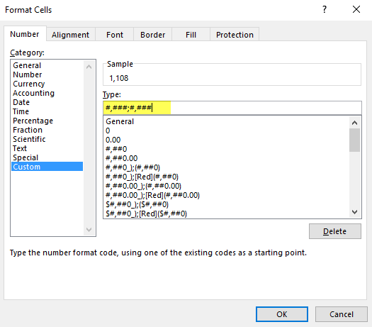
2. Hit Ctrl + 1 to bring up the Format Cells dialog box.
3. Choose “Custom” from the options.
4. In the Type field, I input #,###;#,###.
5. Then I click OK.

After these steps, all the negative numbers appear as positives in the cells, but they’re still negative. If I check the formula bar, the actual value remains unchanged, which means they will still behave like negative numbers in calculations.

I keep in mind that this is just a visual change and for presentation purposes. The underlying values are intact and will still affect formulas as actual negatives.

6. Run a VBA Code to Convert to Positive Numbers

I’ve got a quick trick for my fellow VBA enthusiasts out there. If you encounter a bunch of negative numbers in Excel that you need to flip to positives, there’s no need to do it manually. Here’s a concise VBA code snippet that’ll do the heavy lifting for you:

Sub numberP2N()
    Dim myCell As Range
    For Each myCell In Selection
        If myCell.Value <> "" And IsNumeric(myCell.Value) Then
            myCell.Value = Abs(myCell.Value)
        End If
    Next myCell
End Sub

Just select the cells with the negative numbers, run this macro, and voilà, they’re all positive. Remember, once you run this code, there’s no ‘Ctrl+Z’ to revert, so be sure you’re ready for the change.

Feeling unsure about VBA? Here’s a handy VBA Tutorial that can help you become more comfortable with it. And for those who’ve just started dipping their toes in VBA, check out some useful tips here. Keep coding and keep it cool.

7. Use Power Query to Convert Get Positive Numbers

When I’m faced with the need to convert negative numbers to positive in Excel, I find Power Query to be super handy. Here’s how I do it:

• I start by selecting any cell within the data range that contains the negative numbers I want to work with.

  

• Next, I head over to the Data tab and click on ‘From Table’.

  

• This action transforms my range into a table and brings it up in Power Query Editor.

  

• Here, I just right-click the column in question, select ‘Transform’ and then ‘Absolute Value’ to convert those pesky negatives to positives.

  

• To wrap it up, I hit the Home tab, then ‘Close’ and choose ‘Close and Load’ to finalize everything.

  

For more detailed steps and features, checking out the Power Query Tutorial might be a good idea. It’s quite a game-changer once you get the hang of it.

Conclusion

In our exploration, we’ve uncovered multiple methods to turn those frowns – I mean, negative numbers – upside down. Sure, you could pick your favorite and stick with it, but isn’t it nicer to have options? Remember, each situation might call for a different approach, so having a few tricks up your sleeve isn’t a bad idea.

Now, I’ve shared my insights, but I’m just one person. Maybe you’ve got a slick method I haven’t stumbled upon yet. If so, drop those tips in the comments! It’s not just me who’s eager to learn more, but our whole squad reading this. And hey, if you spread the word to your pals, they might just send a thank-you note your way.