I’ve always found pivot tables to be a game-changer in Excel. They let you analyze complex data sets with ease, and when it comes to diving deeper, calculated fields and items are the secret sauce. Imagine not being limited by the data you have; instead, you create new data points right within your pivot tables through custom calculations. That’s powerful.
So, I was tinkering with a pivot table the other day and decided to add a calculated field to find out the average selling price. It struck me – this isn’t about what’s present in the original data, but rather the insights I can pull out of it. Whether I’m using the ribbon’s Analyze tab or the Insert tab to add a slicer for more interactive reports, Excel skills like these make data analysis not just quick and effective, but also quite enjoyable.
Calculated Field in a Pivot Table
In working with pivot tables in Excel, I often find the need for a calculated field. These fields are particularly handy because they are not pulled directly from the source data; instead, they rely on formulas I define within the pivot table.

If I want to track, say, the commission of a salesperson, a calculated field can be essential. To add one, I click anywhere on the pivot table, which brings up the Analyze and Design tabs. Under Analyze, there’s a Fields, Items, & Sets option that I can use to access calculated fields.

Upon selecting “Calculated Field,” a dialog box opens up. This is where I enter the details of my custom calculation.

- Name: Here’s where I type in what I want to call my calculated field – like “Sales Commission.”
- Formula: This is where I plug in the actual formula using the fields from my data. I have to ensure that my formulas are written correctly.
- Fields: Handy for pulling other data points from my dataset if I need to refer to them in my formula.
A calculated field functions like a virtual column in the pivot table, where it uses the values from the specified fields to carry out its calculations. This lets me create a dynamic summary from my dataset without altering the actual source data. For example, I can easily calculate tax, total sales by quarter, or profit margin. I can also display these as percentages of a total or even rank items to analyze data further. It feels like adding a superpower to my data analysis capabilities!
Calculated Items in a Pivot Table
Calculated items are unique creations within a pivot table. They are not pulled directly from the existing source data but are formed through customized formulas. As with any modifications or enhancements made to data presentation, it’s essential to approach calculated items with a clear understanding of what you aim to achieve and the impact it has on the datasets.
Creating calculated items involves:
- Navigating to the Analyze tab after clicking an item in the pivot table
- Selecting Fields, Items, & Sets
- Opting for Calculated Item
Once selected, a dialogue box pops up where you can input a formula and specify the associated fields and items for the calculation. For example, let’s say I wish to compute the average selling price; I would formulate it as = amount/quantity, inserting the chosen fields and the division operator accordingly.
After pressing OK, this new calculated item will emerge in the pivot table, albeit without any number formatting initially.
Creating calculated items allows analyses like average sales for different time periods. For instance, I might want to calculate the first and second half yearly averages. I just have to input the average formula for the respective months and voilà, the pivot table now displays averages for each half of the year.
It’s imperative, however, to remember that pivot table totals and subtotals account for calculated fields when aggregating. This inclusion could alter the grand row total and grand column total. I noticed this firsthand when my grand totals shifted after inserting calculated items.
To keep the integrity of the original data in check, a keen eye must be maintained for any unintended changes. Should this happen, filtering out calculated items can help retain the accurate representation of the initial data ensemble.
The process is uncomplicated but demands attention to detail, especially when considering the solve order — the sequence in which Excel computes calculated items. It’s an essential aspect to manage carefully as it directly influences the accuracy of the grand total and subtotals in the final output.
Things To Remember
- Modify formulas carefully; omit the 0 when not necessary.
- Use functions without cell references in my formulas.
- Filter out any results skewed by calculated items—check those totals.
- Set the solve order to align with my calculation needs.
- Remember, there are limitations; PivotTables have their own rules.

