Whenever I work with large sets of data in Excel, one of the most common tasks I find myself doing is checking for the existence of a specific value within a range. I’ve learned that the beauty of Excel lies in its powerful functions that make searching through rows and columns not just possible, but also efficient. In particular, I often rely on the COUNTIF and IF functions in tandem—a combo that allows me to quickly ascertain whether a value is present in my dataset.
Using COUNTIF, I count the occurrences of the value across a specified range, and then with the IF function, I evaluate the count to determine an outcome—be it a simple confirmation like “Yes” or “No”, or something more tailored like “Found” or “Not Found.” This method, I’ve found, is an indispensable trick for effective data management. It turns a potentially time-consuming search into just a few clicks and keystrokes, empowering me to focus more on analysis and less on the mechanics of data retrieval.
Check for a Value in a Range
When I’m working with Excel, I sometimes need to see if a specific value exists within a certain range of cells. For example, I have a column full of names, and I want to find out if “GLEN” is one of them. Here’s how I do it:
I start by selecting the cell where I want to display the result—in this case, let’s say cell B1—and type in the IF function.
Next, I include the COUNTIF function within the IF function’s logical test parameter so that Excel will count occurrences of the value “GLEN” within a specified range. This range is my target list of names; let’s say it’s in cells A1 through A10.

Here’s the breakdown of the steps I take:
- Step 1: Type
=IFin cell B1. - Step 2: Insert the
COUNTIFfunction as the logical test. - Step 3: Specify the range A1 where Excel should look for the value.
- Step 4: Inside COUNTIF, use “GLEN” as the criterion.
- Step 5: After COUNTIF, I add
> 0to determine if “GLEN” was found at least once. - Step 6: For the value if true, I use
"Yes". - Step 7: For the value if false, I use
"No".
Then I press Enter. If “GLEN” is indeed within A1, cell B1 proudly displays “Yes”.
Here’s what the final formula looks like:
=IF(COUNTIF(A1:A10,"Glen") > 0,"Yes","No")
This simple method makes it super easy for me to verify the existence of data in large datasets or adjacent cells without manually searching every row and cell value. And if I’m eager to gain a deeper understanding of Excel formulas, I can check out some handy resources like Free Courses: 50 Excel Formulas to Get Smarter than Your Colleagues to boost my skills.
How this Formula Works
I’ll break down this neat formula in simple terms. It’s a combo where I start with COUNTIF to tally if my specific value makes an appearance within the set range.
- Criteria given to
COUNTIFchecks for the value. - Logical test:
COUNTIFoutcome is then compared with 0 using the>(greater than operator).
Then, the IF function waltzes in:
- If the
COUNTIFoutcome is greater than 0, I know the value exists, andIFreturns Yes. - In case
COUNTIFgives me a 0, meaning no show,IFtells me No.
Here’s what the syntax whispers to me:
=IF(COUNTIF(range, criteria) > 0, "Yes", "No")
It’s an efficient way to conduct a logical test and get a return value with minimal fuss.
Check for a Value in a Range Partially
When I need to find a partial match in Excel, especially when dealing with text data, wildcard characters are my go-to. Let’s say I’m skimming through a column for a name that includes “Glen” — but “Glen” could be a part of a longer string.
- I use the asterisk (*) — it’s the wildcard character that stands for any number of characters.
- If I’m looking for a substring anywhere within the cell value, I’ll concatenate the asterisks to my search string.
- Remember, the formula
=IF(COUNTIF(C1:C10,"*" & "Glen" & "*") > 0,"Yes","No")helps check for any instance of “Glen” in the cells C1 through C10, giving a “Yes” if there’s a match and “No” if not.
Here’s how to construct the formula:
- Start with
=IF(COUNTIF( - Specify the range:
C1:C10, - Concatenate the wildcard with the partial value:
"*" & "Glen" & "*", - Define the output for exact match (
> 0) and non-match:),"Yes","No").

This formula is handy because it doesn’t care what comes before or after the name “Glen,” ensuring you can find names like “Glendale” or “BlenGento” just as easily.
Related Formulas
In my work with Excel, I’ve found a few key formulas incredibly handy for different tasks:
- COUNTIF: Essential for counting cells that meet a specific criterion, like finding a particular text within a range.
=COUNTIF(range, "criteria")
- MATCH: Useful for searching for items in a range and returning their position.
=MATCH(lookup_value, lookup_array, [match_type])
- VLOOKUP: Perfect for vertical lookups, retrieving data from a specified column in the same row of the lookup value.
=VLOOKUP(lookup_value, table_array, col_index_num, [range_lookup])
- ISNUMBER: Handy when I need to check if a cell contains a numeric value.
=ISNUMBER(value)
-
Conditional Formatting: I often apply this to visually highlight important data using criteria I define.
-
Google Sheets Formulas: Similar to Excel, Google Sheets supports functions like COUNTIF, MATCH, and VLOOKUP.
Keep in mind, these are just the building blocks. I mix and match them to create more complex formulas tailored to my datasets!


