I remember someone once asking me for help on how to insert a check mark symbol in Excel. It turns out, that’s a common need – especially when managing lists. What you may not know is that there are several ways to do this, catering to different needs and preferences. Whether you’re ticking off tasks, marking attendance, or just like to keep things organized, inserting a check mark can be as simple as a keyboard shortcut or a click on the right font, like Wingdings 2.
Recently, I discovered that apart from the usual methods, Excel offers a whole variety of options for inserting and working with check marks. For instance, you can use the ANSI character code, utilize the convenience of the Windows key, or add some flair to your documents in PowerPoint. Even more so, formatting the check mark to fit the style of your document, like using Calibri for a clean look, or counting how many times the symbol appears in a data range, are all possible and quite straightforward once you know how.
Quick Notes
- Symbol: Use a checkmark from Wingdings font.
- Cell: Apply Wingdings to display the symbol correctly.
- Font Style: Select Wingdings in the Font drop-down.
- Symbol Dialog Box: Access by clicking Symbols on the insert tab.
- Character Code: Enter
252for Wingdings checkmark. - Ribbon: Find Symbols in the Insert tab.
Also, feel free to download this sample file to see how it’s done.
When You Should be Using a Check Mark in Excel
In my spreadsheets, I like to use check mark symbols when I’m:
- Tracking progress in to-do lists
- Indicating tasks I’ve completed
- Confirming items have been reviewed
They’re super handy in Microsoft Excel to visually simplify the status of my work!
1. Keyboard Shortcut to Add a Checkmark
I’ve found that nothing beats a good old keyboard shortcut for speed. Adding a checkmark in Excel? Easy-peasy when you’ve got a shortcut at your fingertips. Just make sure to set your font to Wingdings first, and you can pop a checkmark into your cell quicker than you can say “done.”
Here’s how I do it:
-
On Windows: I just click on the cell where I want my checkmark, hold down the Alt key, and key in 0252 using the numeric keypad.

-
On Mac: It’s just as simple. I select the desired cell, press and hold the Option key, and type 0252. Checkmark appears as if by magic.

And that’s all there is to it! With these shortcuts, I can quickly move on to the next task without missing a beat.
2. Copy Paste a Checkmark Symbol in a Cell
I find the simplest way to get a checkmark into a cell is just by copying and pasting it. Here’s a checkmark you can use: ✓. I just copy it and then go right into Excel and paste it into the cell I want—no need to fiddle with any formulas or shortcuts. Plus, I don’t even have to switch the font—it’s that easy. Want to grab a checkmark yourself? A quick online search gives you plenty to choose from.
3. Insert a Check Mark Directly from Symbols Options
If I need to add a check mark in Excel, I usually head straight to the Symbols options. Here’s how I do it:
-
First things first, I select the cell where the check mark needs to go.
-
Next, I navigate by clicking Insert Tab ➜ Symbols ➜ Symbol.

-
A symbol window pops up. From here, I pick “Wingdings” from the font dropdown menu.
-
Then, in the character code field, I pop in “252”. This action highlights the check mark for me without needing to search for it.

-
After selecting it, I click “Insert”, and bam, it’s right there in the cell, which automagically switches to “Wingdings” style.
And if I’m feeling fancy, I might choose the boxed check mark instead by entering “254”.
Should there be existing text in the cell, I simply edit it (I hit F2) and then follow the same steps to add my check mark. No formula or shortcuts needed, just straight-up insertion. Plus, after getting that check mark in there, I can copy and paste it wherever else I need it throughout my spreadsheet. Easy peasy!
4. Create an AUTOCORRECT to Convert it to a Check Mark
Excel’s handy AUTOCORRECT feature isn’t just for fixing typos. I find it equally powerful for inserting symbols, like check marks. Here’s how I set it up:
- I start by clicking on the File Tab and selecting Excel options.

- From there, I head over to “Proofing” and click to open the AutoCorrect Options.

- In the dialog that pops up, I type in a unique word like CMRK in the “Replace” box – that’s my shortcut for the check mark.
- Next, in the “With:” field, I paste the check mark symbol.

- After clicking OK, I’m all set. Typing CMRK in a cell magically transforms it into a check mark.

Here are some tips I’ve learned along the way:
- The shortcut is case-sensitive, so I usually generate two entries for uppercase and lowercase, just to cover my bases.
- I have to type the shortcut as a standalone word; it won’t convert if it’s part of another word.
- Plus, this autocorrect trick isn’t just for Excel; it works across Office apps, letting me use the same shortcut for a check mark in Word, Outlook, or PowerPoint.
With these steps, inserting check marks becomes a breeze, saving me clicks and time, especially when I’m dealing with extensive lists.
5. Macro to Insert a Checkmark in a Cell
Here’s How This Code Works
When I select cells and execute the code, it circles through each cell, switching the font to “Wingdings” and typing in “ü.” That character corresponds to a checkmark in the “Wingdings” font, so what I get is a neat tick in each cell.
Here’s a simple version of that code:
Sub addCheckMark()
    Dim rng As Range
    For Each rng In Selection
        With rng
            .Font.Name = "Wingdings"
            .Value = "ü"
        End With
    Next rng
End Sub
Make sure to save the macro in your Personal Macro Workbook so you can use it across all your files.
Add Macro Code to QAT
If you, like me, find this macro handy and want quick access to it, adding it to your Quick Access Toolbar (QAT) is a breeze. Here’s what you’ll do:
- Click the small downward arrow on your QAT to open “More Commands.”
- Choose “Macros” from the “Choose Commands From” dropdown.
- Hit “Add>>” to move the macro to the QAT list.
- Click “OK” to finalize.
Now, with just one click, I can run the macro without navigating through menus.
Double-Click Method Using VBA
Maybe you’ve got a spreadsheet and you’d love to check items off with a simple double-click. Here’s a neat trick using VBA:

Private Sub Worksheet_BeforeDoubleClick(ByVal Target As Range, Cancel As Boolean)
    If Target.Column = 2 Then
        Cancel = True
        Target.Font.Name = "Wingdings"
        If Target.Value = "" Then
            Target.Value = "ü"
        Else
            Target.Value = ""
        End If
    End If
End Sub
To set this up, I:
- Right-click the worksheet tab, then “View Code.”
- Paste the above VBA code and close the editor.
- Now any double-click on a cell in column B toggles a checkmark.
What this does is check if the double-clicked cell is in column B. If it’s empty, the code adds a checkmark. If it’s already a check, it clears the cell. Cool, right?

6. Add a Green Check Mark with Conditional Formatting
To make your checklist visually appealing, I find that conditional formatting is a fantastic tool to display a green check mark for completed tasks. Here’s the simple process I follow:
- I start by selecting the cells in my list that will display the check marks upon completion.
- Next, I navigate to Home Tab ➜ Styles ➜ Conditional Formatting ➜ Icon Sets ➜ More Rules. This opens up a new window where the magic happens.
- In this window, I select the green check mark icon. I make sure to check the “Show icon only” box, so that only the symbol is displayed.
+----------------------+---------------+------------------+
|      **Actions**     | **Icon Sets** |   **More Rules** |
+----------------------+---------------+------------------+
| Select Target Cells  | Choose Icons  | Show Icon Only   |
| Enter '1' for Value  |               | Select 'Number'  |
+----------------------+---------------+------------------+
- To set the rule, I input “1” in the number field. This tells Excel to show a green check mark any time I type “1” in the cell.
After applying these settings, all I do is type “1” in any cell in the designated range, and it automatically turns into a vivacious green check mark.

And if I want to copy this conditional formatting to another set of cells, I just use the format painter tool—it’s super handy. You can learn more about it here. It’s quick, it’s easy, and it really brings my checklists to life!
7. Create a Dropdown to Insert a Checkmark
Before adding a dropdown list for checkmarks in Excel, I make sure to have a checkmark ✓ symbol copied to my clipboard for quick use. Here’s how I get interactive checkboxes in place:
- I select the cell where I want my checkbox dropdown to appear.
- I navigate to
Data -> Data Validation. - In the
Data Validationdialog box, under theSettings tab, I chooseListfrom the Allow options. - In the
Sourcebox, I paste the checkmark ✓. If I also need a cross symbol ✖ to toggle between, I add it right after the checkmark, separated by a comma (✓, ✖).
This creates a dropdown where only the checkmark or cross symbol can appear, which simplifies my sheet and makes it more visual.
Additionally, to restrict input to just these symbols, I use the Error Alert tab:
- I check the option
Show error alert after invalid data is entered. - I set a custom message to remind users to select from the dropdown.
Quick Reference:
- Insert a checkmark symbol directly into the dropdown list.
- Disallow other values by customizing an error alert.
- Add multiple symbols such as ✓ and ✖ in the same dropdown for versatility.
Remember: This method ensures an interactive checkbox without the fuss of formulas or repeated copy-pasting.
Further Reading:
- Here’s how I can create an even more dynamic dropdown: How to Create a Dynamic Dropdown List in Excel.
- And for those times when the dropdown needs to change based on another choice, I learned to make a dependent one here: How to Create a Dependent Dropdown List in Excel.
8. Use CHAR Function
Quick INTRO: CHAR Function
To get a tick symbol in Excel, the CHAR function is my buddy. It’s a handy tool when I need Excel to automatically spit out a checkmark based on specific criteria. Let’s say I’ve got a list of tasks and I’m marking them “done” in one column. Instead of manually entering the tick symbol, I let CHAR do the lifting.
Syntax for a quick ref:
CHAR(number)
…how does it work
Imagine this: I type “done” in a cell, and like magic, a checkmark appears in another. That’s CHAR converting numbers to characters right before my eyes. For Excel to show me a checkmark, I simply input 252 into the CHAR function because that’s the number linked to the tick mark in the ANSI standard.
Here’s how to use it in the formula bar:
=CHAR(252)
When I input this, it returns a tick symbol, just the way I like it. Handy, right?
9. Graphical Checkmark
I’ve discovered a super handy feature in Office 365’s Excel. There’s this “Draw” tab on the ribbon, and it’s a game-changer for personalized inputs.
- First off, there’s a variety of pens and markers to choose from.
- Simply by drawing a checkmark, Excel converts it into a graphic.
| Tool | Use |
|---|---|
| Pen/Marker | Draw a checkmark or other symbols. |
| Eraser | Remove drawings or mistakes. |
What I love about drawing a checkmark directly:
- It retains the graphic format across different versions of Excel.
- No need to bother with Wingdings or Segoe UI Symbol fonts.
- Bypass the UNICHAR function or memorizing Unicode codes.

It’s like having a digital whiteboard right in my spreadsheet. The “Draw” tab is seriously worth exploring, it takes your spreadsheet game to a whole new level!
10. Use Checkbox as a Checkmark in a Cell
Adding checkboxes in Excel is super handy for making interactive to-do lists. Unlike a checkmark, which lives right in a cell, a checkbox hovers on top. If I’m deleting cells, my checkboxes stick around—they’re like cool floaty reminders that don’t get swept away with cell content. Checkboxes give me that satisfying click to cross things off without mixing up with my data.
Here’s how I get it done:
- Insert a checkbox from the Controls section in the Developer tab.
- Draw it over the cell where I want that visual tick.
- Link the checkbox to a cell to get that true/false value, which is awesome for tracking stuff.
And guess what? There’s a bunch more I can do with checkboxes. If I’ve piqued your curiosity, check this out for a deep dive into using checkboxes like a pro.
11. Insert a Checkmark (Online)
In my experience with Microsoft 365’s Excel file, inserting a checkmark online can be a bit tricky since the traditional “Wingdings” font and CHAR function don’t do the trick. But no worries, I’ve got a workaround that involves adding an app to Online Excel which makes it so much easier. Let me show you the steps:
- Open your Excel file in the online app.
- Head over to ‘Insert’ and choose ‘Office Add-ins’.
- Look for an add-in that provides symbol insertion functionality.
- Add it to your Excel, and there you should find checkmark symbols to insert.
Here’s a sample file, which I recommend downloading to see how this works in action.
Some of the IMPORTANT Points YOU need to learn
1. Formatting a Checkmark
When I’m validating data and need my checkmarks to stand out, here’s what I do:
- Bold or italicize the checkmark for emphasis.
- Switch up the checkmark’s color to match my theme or highlight its status.
- Adjust the font size bigger for visibility or smaller to keep it unobtrusive.
- Underline for that extra pop or to signify something special.
2. Deleting a Checkmark
For those times when a checkmark has gotta go, I just select the cell and tap that delete key. Now, if there’s text in there too, it gets a little different:
- I can hit F2 to edit the cell directly and show that checkmark the exit.
- Or use the nifty find and replace to swap out the checkmark for nada. For example, like this.
3. Count Checkmarks
So, let’s say I’m curious about how many checkmarks I’ve got across my sheet. Here’s the formula magic I use:
=COUNTIF(G3:G9, CHAR(252))
This neat little formula combines COUNTIF with CHAR to tell me exactly what I need to know. The CHAR part gets the checkmark, and COUNTIF takes care of the tally. And, if you’re itching to try it out for yourself, snag the sample file right here and give it a whirl.
In the end
I’ve been tapping away at Excel, working through lists and adding check marks like they’re going out of style. It’s amazing how a small tick can give such a sense of accomplishment. Whether it’s using conditional formatting for that extra flair or the good ol’ copy-paste method for efficiency, each approach has its charm.
- Conditional Formatting: Oh, how I love the colors and automation.
- Copy-Paste: Quick and straightforward—just my style.
And hey, I’m curious about your experiences. Drop me a comment below with your go-to method. Sharing is caring, so pass this knowledge along to your pals too—I bet they’ll thank you later!


